Plotting Interaction Effects
Interaction effects can be plotted using the included
plot_interaction() function. This function takes a fitted
model object and the names of the two variables that are interacting.
The function will plot the interaction effect of the two variables,
where:
- The x-variable is plotted on the x-axis.
- The y-variable is plotted on the y-axis.
- The z-variable determines at which points the effect of x on y is plotted.
The function will also plot the 95% confidence interval for the
interaction effect. Note that the vals_z argument (as well
as the values of x) are scaled by the mean and standard
deviation of the variables. Unless the rescale argument is
set to FALSE.
Here is a simple example using the double-centering approach:
m1 <- "
# Outer Model
X =~ x1 + x2 + x3
Z =~ z1 + z2 + z3
Y =~ y1 + y2 + y3
# Inner Model
Y ~ X + Z + X:Z
"
est1 <- modsem(m1, data = oneInt)
plot_interaction(x = "X", z = "Z", y = "Y",
vals_z = -3:3, model = est1)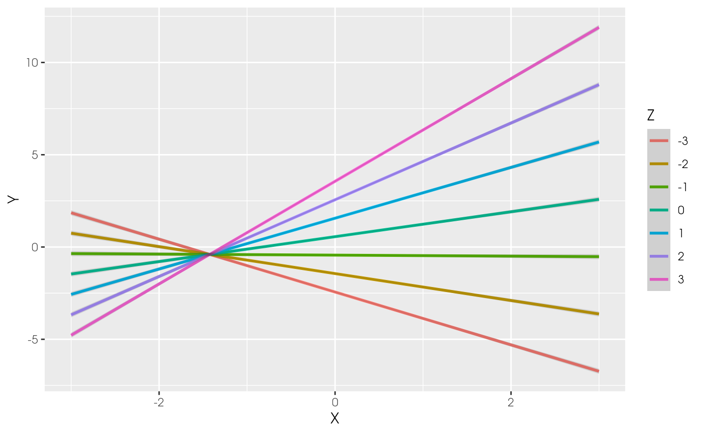
Here is a different example using the lms approach in
the theory of planned behavior model:
tpb <- "
# Outer Model (Based on Hagger et al., 2007)
ATT =~ att1 + att2 + att3 + att4 + att5
SN =~ sn1 + sn2
PBC =~ pbc1 + pbc2 + pbc3
INT =~ int1 + int2 + int3
BEH =~ b1 + b2
# Inner Model (Based on Steinmetz et al., 2011)
INT ~ ATT + SN + PBC
BEH ~ INT + PBC
BEH ~ PBC:INT
"
est2 <- modsem(tpb, TPB, method = "lms")
plot_interaction(x = "INT", z = "PBC", y = "BEH",
vals_z = c(-0.5, 0.5), model = est2)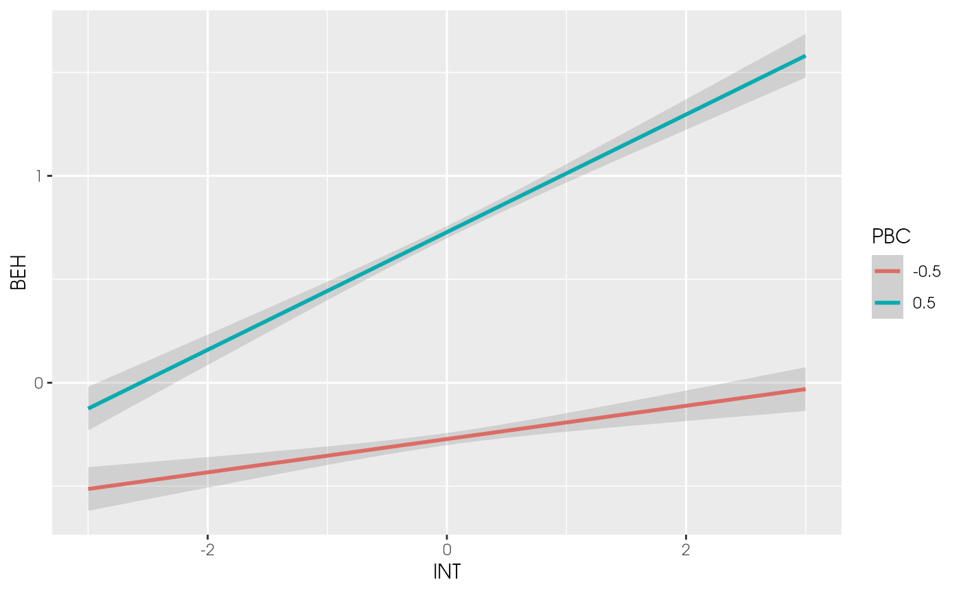
Plotting Johnson-Neyman Regions
The plot_jn() function can be used to plot
Johnson-Neyman regions for a given interaction effect. This function
takes a fitted model object, the names of the two variables that are
interacting, and the name of the interaction effect. The function will
plot the Johnson-Neyman regions for the interaction effect.
The plot_jn() function will also plot the 95% confidence
interval for the interaction effect.
x is the name of the x-variable, z is the
name of the z-variable, and y is the name of the
y-variable. model is the fitted model object. The argument
min_z and max_z are used to specify the range
of values for the moderating variable.
Here is an example using the ca approach in the
Holzinger-Swineford (1939) dataset:
m1 <- '
visual =~ x1 + x2 + x3
textual =~ x4 + x5 + x6
speed =~ x7 + x8 + x9
visual ~ speed + textual + speed:textual
'
est1 <- modsem(m1, data = lavaan::HolzingerSwineford1939, method = "ca")
plot_jn(x = "speed", z = "textual", y = "visual", model = est1, max_z = 6)
#> Johnson-Neyman regions:
#> When textual <= -1.52, the direct effect of speed is not significant (p >= .05).
#> When textual is between -1.52 and 5.20, the direct effect of speed is p < .05.
#> When textual >= 5.20, the direct effect of speed is not significant (p >= .05).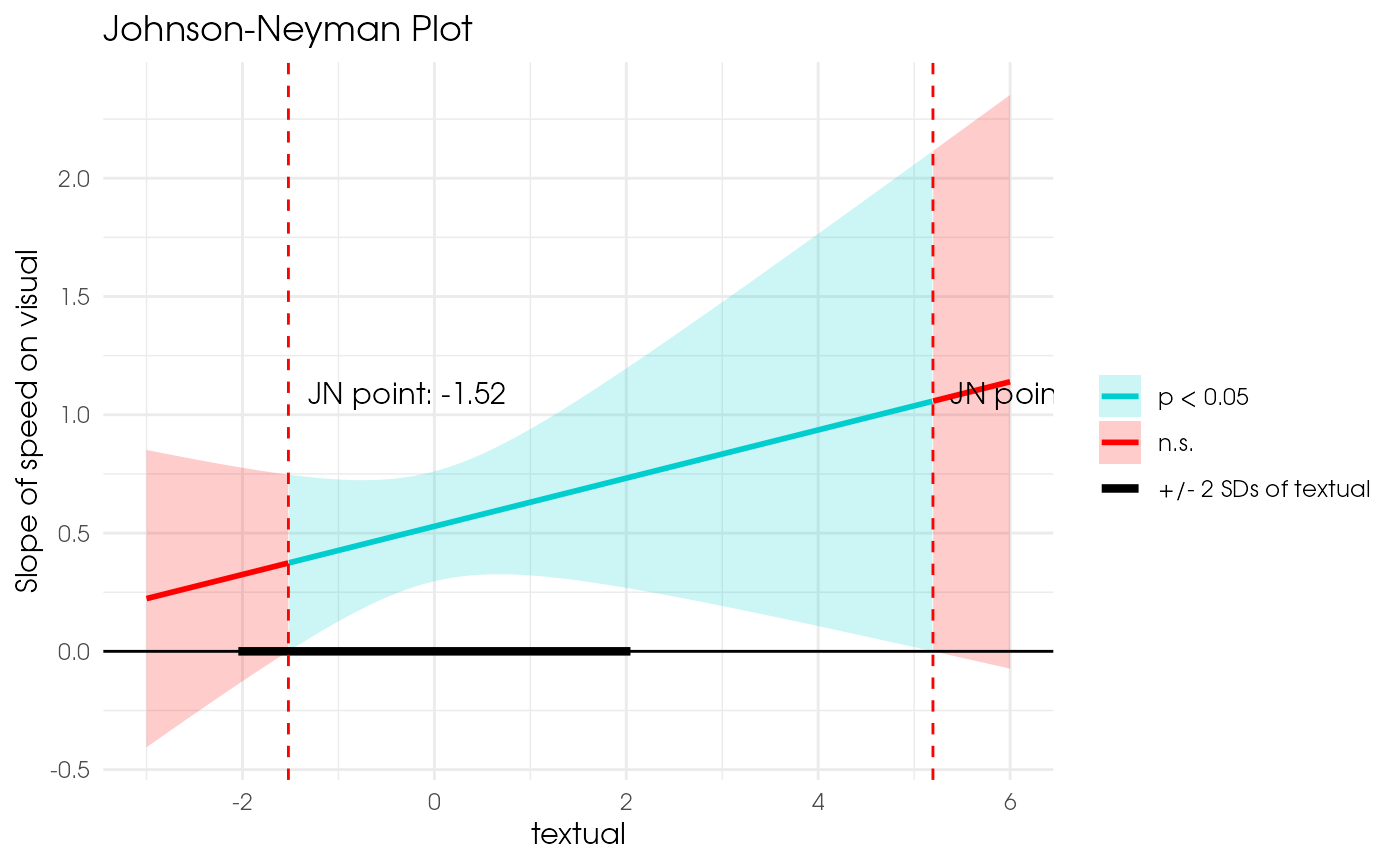
Here is another example using the qml approach in the
theory of planned behavior model:
tpb <- "
# Outer Model (Based on Hagger et al., 2007)
ATT =~ att1 + att2 + att3 + att4 + att5
SN =~ sn1 + sn2
PBC =~ pbc1 + pbc2 + pbc3
INT =~ int1 + int2 + int3
BEH =~ b1 + b2
# Inner Model (Based on Steinmetz et al., 2011)
INT ~ ATT + SN + PBC
BEH ~ INT + PBC
BEH ~ PBC:INT
"
est2 <- modsem(tpb, TPB, method = "qml")
plot_jn(x = "INT", z = "PBC", y = "BEH", model = est2,
min_z = -1.5, max_z = -0.5)
#> Johnson-Neyman regions:
#> When PBC <= -1.24, the direct effect of INT is p < .05.
#> When PBC is between -1.24 and -0.67, the direct effect of INT is not significant (p >= .05).
#> When PBC >= -0.67, the direct effect of INT is p < .05.
#> Warning: modsem->plotJN_Group():
#> Truncating SD-range on the right and left!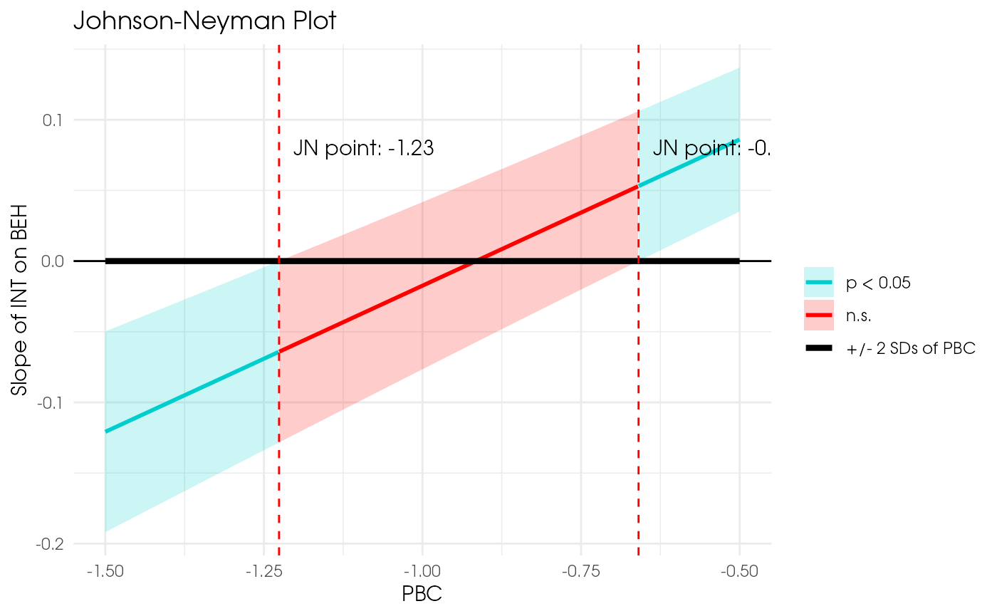
Plotting (3D) Surface Plots
The plot_surface() function can be used to plot 3D
surface plots for a given interaction effect. This function takes a
fitted model object, the names of the two variables that are
interacting, and the name of the dependent variable. The function will
plot the 3D surface plot for the interaction effect.
tpb <- "
# Outer Model (Based on Hagger et al., 2007)
ATT =~ att1 + att2 + att3 + att4 + att5
SN =~ sn1 + sn2
PBC =~ pbc1 + pbc2 + pbc3
INT =~ int1 + int2 + int3
BEH =~ b1 + b2
# Inner Model (Based on Steinmetz et al., 2011)
INT ~ ATT + SN + PBC
BEH ~ INT + PBC
BEH ~ PBC:INT
"
est2 <- modsem(tpb, TPB, method = "qml")
plot_surface(x = "INT", z = "PBC", y = "BEH", model = est2)Quadratic Effects and Response Surface Models
As of version 1.0.13, modsem also handles
quadratic effects when plotting interaction using the
plot_interaction() and plot_surface()
functions. Here we can see an example using some generated data for a
model with two quadratic effects, and a single interaction effect. The
model is equivalent to a typical response surface regression.
Generating Data
set.seed(2934269)
var_X <- 1
var_Z <- 1
cov_X_Z <- 0.2
zeta_Y <- 0.4
gamma_Y_X <- 0
gamma_Y_Z <- 0
gamma_Y_XZ <- 1
gamma_Y_ZZ <- 3 # exclude for now
gamma_Y_XX <- -1 # exclude for now
lambda_1 <- 1
lambda_2 <- .7
lambda_3 <- .8
epsilon <- 0.2
beta_1 <- 1.2
beta_2 <- 0.8
beta_3 <- 1.5
N <- 1500
residual <- \(epsilon) rnorm(N, sd = sqrt(epsilon))
create_ind <- \(lv, beta, lambda, epsilon) beta + lambda * lv + residual(epsilon)
Phi <- matrix(c(var_X, cov_X_Z,
cov_X_Z, var_Z), nrow = 2)
XI <- mvtnorm::rmvnorm(N, sigma = Phi)
X <- XI[, 1]
Z <- XI[, 2]
Y <-
gamma_Y_X * X +
gamma_Y_Z * Z +
gamma_Y_XZ * X * Z +
gamma_Y_XX * X * X +
gamma_Y_ZZ * Z * Z +
residual(zeta_Y)
x1 <- create_ind(X, beta_1, lambda_1, epsilon)
x2 <- create_ind(X, beta_2, lambda_2, epsilon)
x3 <- create_ind(X, beta_3, lambda_2, epsilon)
z1 <- create_ind(Z, beta_1, lambda_1, epsilon)
z2 <- create_ind(Z, beta_2, lambda_2, epsilon)
z3 <- create_ind(Z, beta_3, lambda_2, epsilon)
y1 <- create_ind(Y, beta_1, lambda_1, epsilon)
y2 <- create_ind(Y, beta_2, lambda_2, epsilon)
y3 <- create_ind(Y, beta_2, lambda_2, epsilon)
data.sim <- data.frame(
x1, x2, x3,
z1, z2, z3,
y1, y2, y3
)Fitting Model
Here we fit the model using the QML approach.
model <- '
X =~ x1 + x2 + x3
Z =~ z1 + z2 + z3
Y =~ y1 + y2 + y3
Y ~ X + Z + X:X + Z:Z + X:Z
'
est3 <- modsem(model, data = data.sim, method = "qml")2D Plot
Here we can see a two dimensional plot, where the slope of
X no longer is constant at a given value of Z,
since X has an interaction effect with itself.
plot_interaction(x = "X", z = "Z", y = "Y", model = est3, vals_z = c(-1, 0, 1))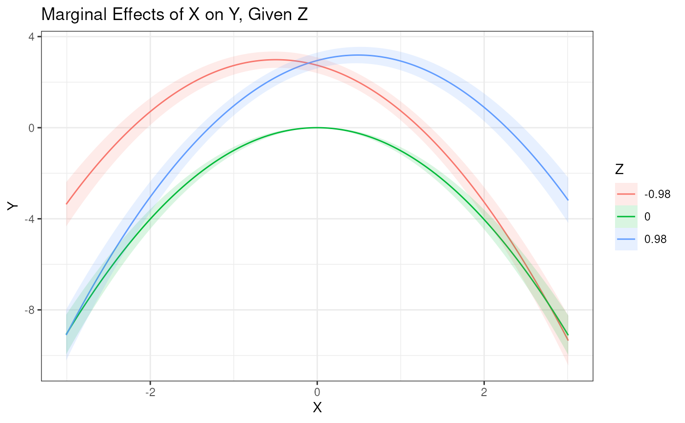
3D (Response Surface) Plot
Here we can see a three-dimensional surface plot.
plot_surface(x = "X", z = "Z", y = "Y", model = est3)