Plot Interaction Effect Using the Johnson-Neyman Technique

This function plots the simple slopes of an interaction effect across different values of a moderator variable using the Johnson-Neyman technique. It identifies regions where the effect of the predictor on the outcome is statistically significant.

Usage

plot_jn(
  x,
  z,
  y,
  model,
  min_z = -3,
  max_z = 3,
  sig.level = 0.05,
  alpha = 0.2,
  detail = 1000,
  sd.line = 2,
  standardized = FALSE,
  xz = NULL,
  greyscale = FALSE,
  plot.jn.points = TRUE,
  type = c("direct", "indirect", "total"),
  mc.quantiles = FALSE,
  mc.reps = 10000,
  ...
)

Arguments

x: The name of the predictor variable (as a character string).
z: The name of the moderator variable (as a character string).
y: The name of the outcome variable (as a character string).
model: A fitted model object of class modsem_da, modsem_mplus, modsem_pi, or lavaan.
min_z: The minimum value of the moderator variable z to be used in the plot (default is -3). It is relative to the mean of z.
max_z: The maximum value of the moderator variable z to be used in the plot (default is 3). It is relative to the mean of z.
sig.level: The alpha-criterion for the confidence intervals (default is 0.05).
alpha: alpha setting used in ggplot (i.e., the opposite of opacity)
detail: The number of generated data points to use for the plot (default is 1000). You can increase this value for smoother plots.
sd.line: A thick black line showing +/- sd.line * sd(z). NOTE: This line will be truncated by min_z and max_z if the sd.line falls outside of [min_z, max_z].
standardized: Should coefficients be standardized beforehand?
xz: The name of the interaction term. If not specified, it will be created using x and z.
greyscale: Logical. If TRUE the plot is plotted in greyscale.
plot.jn.points: Logical. If TRUE, omit the numeric annotations for the JN-points from the plot.
type: Which effect to display. One of "direct", "indirect", or "total".
mc.quantiles: Should JN quantiles be calculated using Monte-Carlo estimates?
mc.reps: Number of Monte Carlo replicates used to approximate the confidence bands when mc.quantile is TRUE and/or type is "indirect" or "total".
...: Additional arguments (currently not used).

Value

A ggplot object showing the interaction plot with regions of significance.

Details

The function calculates the simple slopes of the predictor variable x on the outcome variable y at different levels of the moderator variable z. It uses the Johnson-Neyman technique to identify the regions of z where the effect of x on y is statistically significant.

When plotting indirect or total effects, the function relies on Monte Carlo draws from the estimated sampling distribution of the parameters to approximate the conditional effect and its confidence interval across the moderator range.

It extracts the necessary coefficients and variance-covariance information from the fitted model object. The function then computes the critical t-value and solves the quadratic equation derived from the t-statistic equation to find the Johnson-Neyman points.

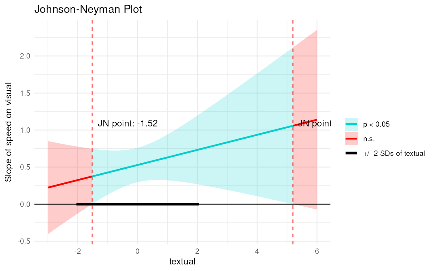
The plot displays:

The estimated simple slopes across the range of z.
Confidence intervals around the slopes.
Regions where the effect is significant (shaded areas).
Vertical dashed lines indicating the Johnson-Neyman points.
Text annotations providing the exact values of the Johnson-Neyman points.

Examples

# \dontrun{
library(modsem)

m1 <-  '
  visual  =~ x1 + x2 + x3
  textual =~ x4 + x5 + x6
  speed   =~ x7 + x8 + x9

  visual ~ speed + textual + speed:textual
'

est <- modsem(m1, data = lavaan::HolzingerSwineford1939, method = "ca")
plot_jn(x = "speed", z = "textual", y = "visual", model = est, max_z = 6)
#> Johnson-Neyman regions:
#>   When textual <= -1.52, the direct effect of speed is not significant (p >= .05).
#>   When textual is between -1.52 and 5.20, the direct effect of speed is p < .05.
#>   When textual >= 5.20, the direct effect of speed is not significant (p >= .05).

# }