Simple Slopes Analysis
Simple slope effects can be plotted using the included
plot_interaction() function. This function takes a fitted
model object and the names of the two variables that are interacting.
The function will plot the interaction effect of the two variables,
where:
- The x-variable is plotted on the x-axis.
- The y-variable is plotted on the y-axis.
- The z-variable determines at which points the effect of x on y is plotted.
The function will also plot the 95% confidence interval for the
interaction effect. Note that the vals_z argument (as well
as the values of x) are scaled by the mean and standard
deviation of the variables. Unless the rescale argument is
set to FALSE.
Here is a simple example using the double-centering approach:
m1 <- "
# Outer Model
  X =~ x1
  X =~ x2 + x3
  Z =~ z1 + z2 + z3
  Y =~ y1 + y2 + y3

# Inner Model
  Y ~ X + Z + X:Z
"
est1 <- modsem(m1, data = oneInt)
plot_interaction(x = "X", z = "Z", y = "Y", vals_z = c(-1, 1), model = est1)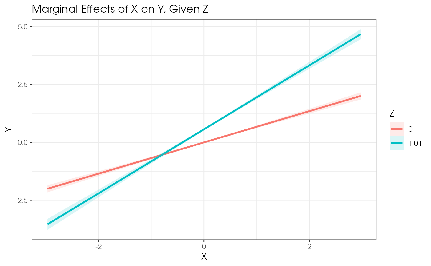
If you want to see the numerical values of the simple slopes, you can
use the simple_slopes() function:
m1 <- "
# Outer Model
  X =~ x1
  X =~ x2 + x3
  Z =~ z1 + z2 + z3
  Y =~ y1 + y2 + y3

# Inner Model
  Y ~ X + Z + X:Z
"

est1 <- modsem(m1, data = oneInt)
simple_slopes(x = "X", z = "Z", y = "Y", vals_z = c(-1, 1), model = est1)
#>
#> Difference test of Y~X|Z at Z = -1.01 and 1.01:
#> ┌───────────┬───────────┬─────────┬─────────┬───────────────┐
#> │Difference │ Std.Error │ z.value │ p.value │ Conf.Interval │
#> ╞═══════════╪═══════════╪═════════╪═════════╪═══════════════╡
#> │      1.42 │      0.05 │   26.36 │   0.000 │  [1.31, 1.52] │
#> └───────────┴───────────┴─────────┴─────────┴───────────────┘
#>
#> Effect of Y~X|Z given values of Z:
#> ┌───────┬────────┬───────────┬─────────┬─────────┬────────────────┐
#> │   Y~X │      Z │ Std.Error │ z.value │ p.value │  Conf.Interval │
#> ╞═══════╪════════╪═══════════╪═════════╪═════════╪════════════════╡
#> │ -0.03 │  -1.01 │      0.04 │   -0.88 │   0.377 │  [-0.11, 0.04] │
#> │  1.38 │   1.01 │      0.04 │   36.34 │   0.000 │  [ 1.31, 1.46] │
#> └───────┴────────┴───────────┴─────────┴─────────┴────────────────┘
#>
#>
#> Predicted Y, given Z = -1.01:
#> ┌───────┬─────────────┬───────────┬─────────┬─────────┬─────────────────┐
#> │     X │ Predicted Y │ Std.Error │ z.value │ p.value │   Conf.Interval │
#> ╞═══════╪═════════════╪═══════════╪═════════╪═════════╪═════════════════╡
#> │ -2.97 │       -0.47 │      0.11 │   -4.17 │   0.000 │  [-0.69, -0.25] │
#> │ -1.98 │       -0.50 │      0.08 │   -6.55 │   0.000 │  [-0.65, -0.35] │
#> │ -0.99 │       -0.53 │      0.04 │  -12.33 │   0.000 │  [-0.62, -0.45] │
#> │  0.00 │       -0.57 │      0.03 │  -21.61 │   0.000 │  [-0.62, -0.51] │
#> │  0.99 │       -0.60 │      0.05 │  -12.56 │   0.000 │  [-0.69, -0.50] │
#> │  1.98 │       -0.63 │      0.08 │   -7.76 │   0.000 │  [-0.79, -0.47] │
#> │  2.97 │       -0.66 │      0.12 │   -5.67 │   0.000 │  [-0.89, -0.43] │
#> └───────┴─────────────┴───────────┴─────────┴─────────┴─────────────────┘
#>
#>
#> Predicted Y, given Z =  1.01:
#> ┌───────┬─────────────┬───────────┬─────────┬─────────┬─────────────────┐
#> │     X │ Predicted Y │ Std.Error │ z.value │ p.value │   Conf.Interval │
#> ╞═══════╪═════════════╪═══════════╪═════════╪═════════╪═════════════════╡
#> │ -2.97 │       -3.54 │      0.12 │  -29.48 │   0.000 │  [-3.78, -3.31] │
#> │ -1.98 │       -2.17 │      0.08 │  -25.94 │   0.000 │  [-2.34, -2.01] │
#> │ -0.99 │       -0.80 │      0.05 │  -16.30 │   0.000 │  [-0.90, -0.71] │
#> │  0.00 │        0.57 │      0.03 │   21.61 │   0.000 │  [ 0.51,  0.62] │
#> │  0.99 │        1.93 │      0.04 │   45.91 │   0.000 │  [ 1.85,  2.02] │
#> │  1.98 │        3.30 │      0.08 │   43.74 │   0.000 │  [ 3.16,  3.45] │
#> │  2.97 │        4.67 │      0.11 │   41.84 │   0.000 │  [ 4.45,  4.89] │
#> └───────┴─────────────┴───────────┴─────────┴─────────┴─────────────────┘
The simple_slopes() function returns a
simple_slopes object. It only has two methods/generics:
print.simple_slopes(), which prints the simple slopes in a
easy-to-read format and as.data.frame.simple_slopes(). The
print() method will not only print the predicted values,
but also significance tests for the difference between the slope at the
lowest value of z and the slope at the highest value of
z, as well as significance tests for the slope of
x at the different values of vals_z.
In the example above, we can see that there is a significant
difference between the slope at at -1 * sd(Z) and
+1 * sd(Z). Note that by default vals_z is
rescaled by the mean and standard deviation of the variable, unless
rescale = FALSE is set. This means that the values of
vals_z are interpreted as standard deviations from the mean
of Z.
If you want to extract the simple slopes as a
data.frame, you can use the as.data.frame()
function:
m1 <- "
# Outer Model
  X =~ x1
  X =~ x2 + x3
  Z =~ z1 + z2 + z3
  Y =~ y1 + y2 + y3

# Inner Model
  Y ~ X + Z + X:Z
"

est1 <- modsem(m1, data = oneInt)
slopes <- simple_slopes(x = "X", z = "Z", y = "Y",
                        vals_z = c(0, 1), model = est1)
as.data.frame(slopes)
#>       vals_x   vals_z  predicted  std.error   z.value       p.value   ci.upper
#> 1  -2.971371 0.000000 -2.0043502 0.07897710 -25.37888 4.315156e-142 -1.8495579
#> 2  -1.980914 0.000000 -1.3362335 0.05265140 -25.37888 4.315156e-142 -1.2330386
#> 3  -0.990457 0.000000 -0.6681167 0.02632570 -25.37888 4.315156e-142 -0.6165193
#> 4   0.000000 0.000000  0.0000000 0.00000000       NaN           NaN  0.0000000
#> 5   0.990457 0.000000  0.6681167 0.02632570  25.37888 4.315156e-142  0.7197142
#> 6   1.980914 0.000000  1.3362335 0.05265140  25.37888 4.315156e-142  1.4394283
#> 7   2.971371 0.000000  2.0043502 0.07897710  25.37888 4.315156e-142  2.1591425
#> 8  -2.971371 1.008084 -3.5419756 0.12016033 -29.47708 5.663689e-191 -3.3064657
#> 9  -1.980914 1.008084 -2.1729189 0.08376085 -25.94194 2.242005e-148 -2.0087506
#> 10 -0.990457 1.008084 -0.8038622 0.04930659 -16.30334  9.343915e-60 -0.7072230
#> 11  0.000000 1.008084  0.5651945 0.02615878  21.60631 1.566928e-103  0.6164648
#> 12  0.990457 1.008084  1.9342513 0.04213439  45.90671  0.000000e+00  2.0168332
#> 13  1.980914 1.008084  3.3033080 0.07552626  43.73721  0.000000e+00  3.4513367
#> 14  2.971371 1.008084  4.6723647 0.11167366  41.83945  0.000000e+00  4.8912411
#>      ci.lower
#> 1  -2.1591425
#> 2  -1.4394283
#> 3  -0.7197142
#> 4   0.0000000
#> 5   0.6165193
#> 6   1.2330386
#> 7   1.8495579
#> 8  -3.7774855
#> 9  -2.3370871
#> 10 -0.9005013
#> 11  0.5139243
#> 12  1.8516694
#> 13  3.1552792
#> 14  4.4534884