Plot Interaction Effects in a SEM Model — plot

This function creates an interaction plot of the outcome variable (y) as a function of a focal predictor (x) at multiple values of a moderator (z). It is designed for use with structural equation modeling (SEM) objects (e.g., those from modsem). Predicted means (or predicted individual values) are calculated via simple_slopes, and then plotted with ggplot2 to display multiple regression lines and confidence/prediction bands.

Usage

plot_interaction(
  x,
  z,
  y,
  model,
  vals_x = seq(-3, 3, 0.001),
  vals_z,
  alpha_se = 0.15,
  digits = 2,
  ci_width = 0.95,
  ci_type = "confidence",
  rescale = TRUE,
  standardized = FALSE,
  xz = NULL,
  greyscale = FALSE,
  ...
)

Arguments

x: A character string specifying the focal predictor (x-axis variable).
z: A character string specifying the moderator variable.
y: A character string specifying the outcome (dependent) variable.
model: An object of class modsem_pi, modsem_da, modsem_mplus, or possibly a lavaan object. Must be a fitted SEM model containing paths for y ~ x + z + x:z.
vals_x: A numeric vector of values at which to compute and plot the focal predictor x. The default is seq(-3, 3, .001), which provides a relatively fine grid for smooth lines. If rescale=TRUE, these values are in standardized (mean-centered and scaled) units, and will be converted back to the original metric in the internal computation of predicted means.
vals_z: A numeric vector of values of the moderator z at which to draw separate regression lines. Each distinct value in vals_z defines a separate group (plotted with a different color). If rescale=TRUE, these values are also assumed to be in standardized units.
alpha_se: A numeric value in \([0, 1]\) specifying the transparency of the confidence/prediction interval ribbon. Default is 0.15.
digits: An integer specifying the number of decimal places to which the moderator values (z) are rounded for labeling/grouping in the plot.
ci_width: A numeric value in \((0,1)\) indicating the coverage of the confidence (or prediction) interval. The default is 0.95 for a 95% interval.
ci_type: A character string specifying whether to compute "confidence" intervals (for the mean of the predicted values, default) or "prediction" intervals (which include residual variance).
rescale: Logical. If TRUE (default), vals_x and vals_z are interpreted as standardized units, which are mapped back to the raw scale before computing predictions. If FALSE, vals_x and vals_z are taken as raw-scale values directly.
standardized: Should coefficients be standardized beforehand?
xz: A character string specifying the interaction term (x:z). If NULL, the term is created automatically as paste(x, z, sep = ":"). Some SEM backends may handle the interaction term differently (for instance, by removing or modifying the colon), and this function attempts to reconcile that internally.
greyscale: Logical. If TRUE the plot is plotted in greyscale.
...: Additional arguments passed on to simple_slopes.

Value

A ggplot object that can be further customized (e.g., with additional + theme(...) layers). By default, it shows lines for each moderator value and a shaded region corresponding to the interval type (confidence or prediction).

Details

Computation Steps:

Calls simple_slopes to compute the predicted values of y at the specified grid of x and z values.
Groups the resulting predictions by unique z-values (rounded to digits) to create colored lines.
Plots these lines using ggplot2, adding ribbons for confidence (or prediction) intervals, with transparency controlled by alpha_se.

Interpretation: Each line in the plot corresponds to the regression of y on x at a given level of z. The shaded region around each line (ribbon) shows either the confidence interval for the predicted mean (if ci_type = "confidence") or the prediction interval for individual observations (if ci_type = "prediction"). Where the ribbons do not overlap, there is evidence that the lines differ significantly over that range of x.

Examples

# \dontrun{
library(modsem)

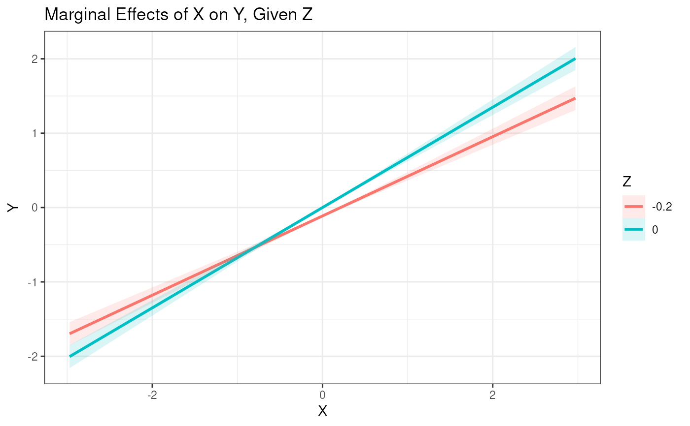
# Example 1: Interaction of X and Z in a simple SEM
m1 <- "
# Outer Model
  X =~ x1 + x2 + x3
  Z =~ z1 + z2 + z3
  Y =~ y1 + y2 + y3

# Inner Model
  Y ~ X + Z + X:Z
"
est1 <- modsem(m1, data = oneInt)

# Plot interaction using a moderate range of X and two values of Z
plot_interaction(x = "X", z = "Z", y = "Y", xz = "X:Z",
                 vals_x = -3:3, vals_z = c(-0.2, 0), model = est1)


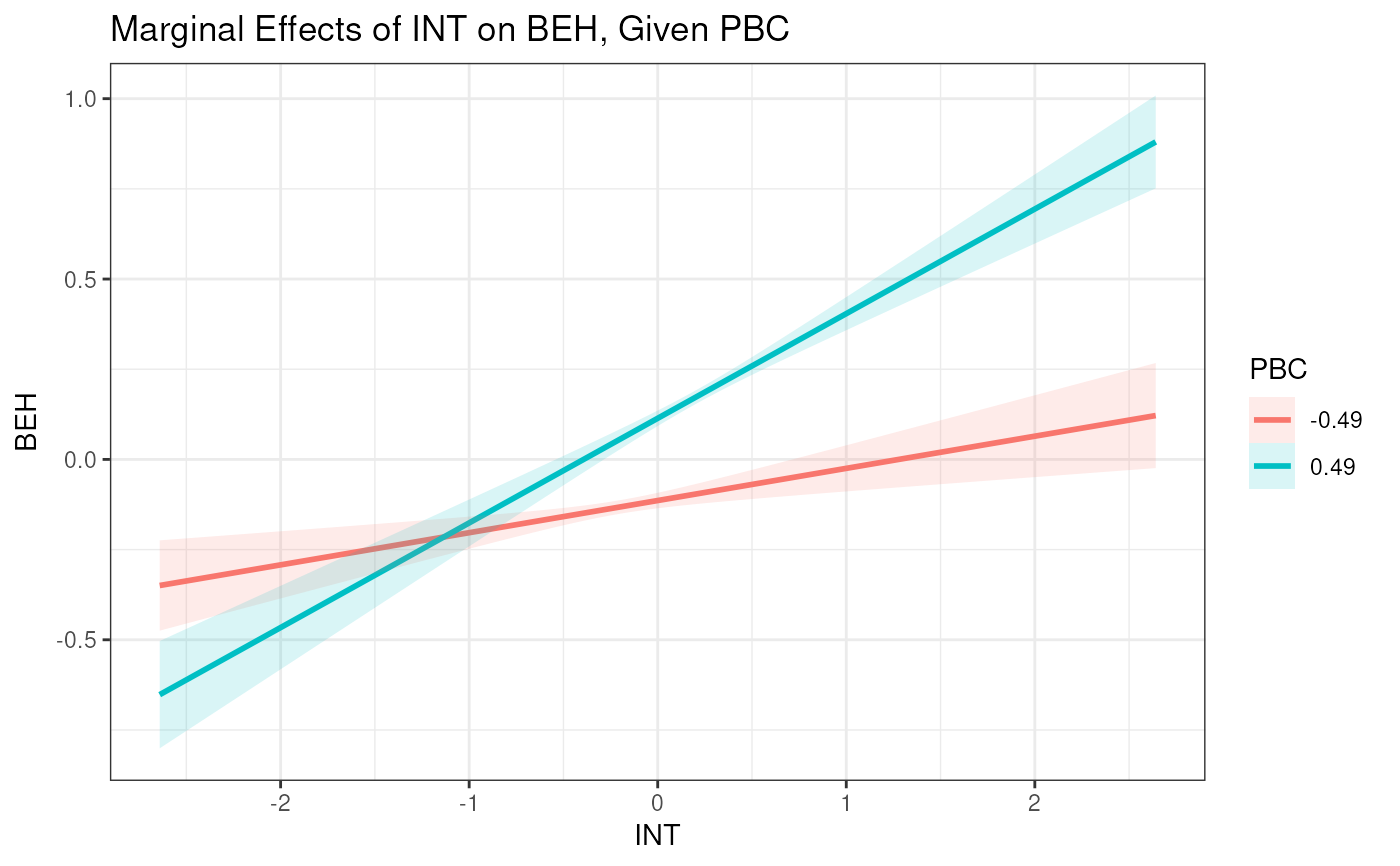
# Example 2: Interaction in a theory-of-planned-behavior-style model
tpb <- "
# Outer Model
  ATT =~ att1 + att2 + att3 + att4 + att5
  SN  =~ sn1 + sn2
  PBC =~ pbc1 + pbc2 + pbc3
  INT =~ int1 + int2 + int3
  BEH =~ b1 + b2

# Inner Model
  INT ~ ATT + SN + PBC
  BEH ~ INT + PBC
  BEH ~ PBC:INT
"
est2 <- modsem(tpb, data = TPB, method = "lms", nodes = 32)

# Plot with custom Z values and a denser X grid
plot_interaction(x = "INT", z = "PBC", y = "BEH",
                 xz = "PBC:INT",
                 vals_x = seq(-3, 3, 0.01),
                 vals_z = c(-0.5, 0.5),
                 model = est2)

# }